Universe by tidyverse.

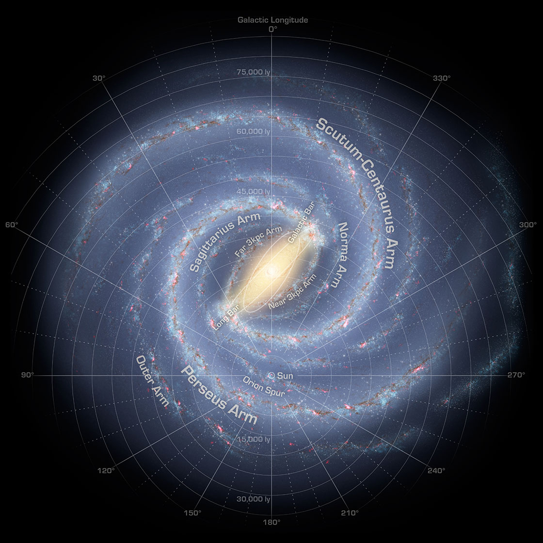
Image by NASA/JPL-Caltech/R. Hurt

In celebration of my first appearance on R-Bloggers

There is no denying that some of the most awe-inspiring photos ever taken can be found in astrophotography. In my low-cost attempt at capturing that magic a few years ago, I posted an image of a procedurally generated Milky Way. Since then, the same methodology has been applied to harmonograph. Today, sit tight because our mission is to document my journey to infinity and beyond.

The idea is simple enough. Structurally, the Milky Way consists of a couple of spiral arms spinning around its center, all of which are in turn made up of numerous teeny-tiny little stars. In the absence of a space telescope, how can we create something that looks reasonably close to the galaxy? Fortunately, we have a few pretty powerful tools at our disposal (specifically, R and tidyverse/ggplot). Note that the focus here is aesthetic pleasingness rather than scientific accuracy.

Spiral Arms

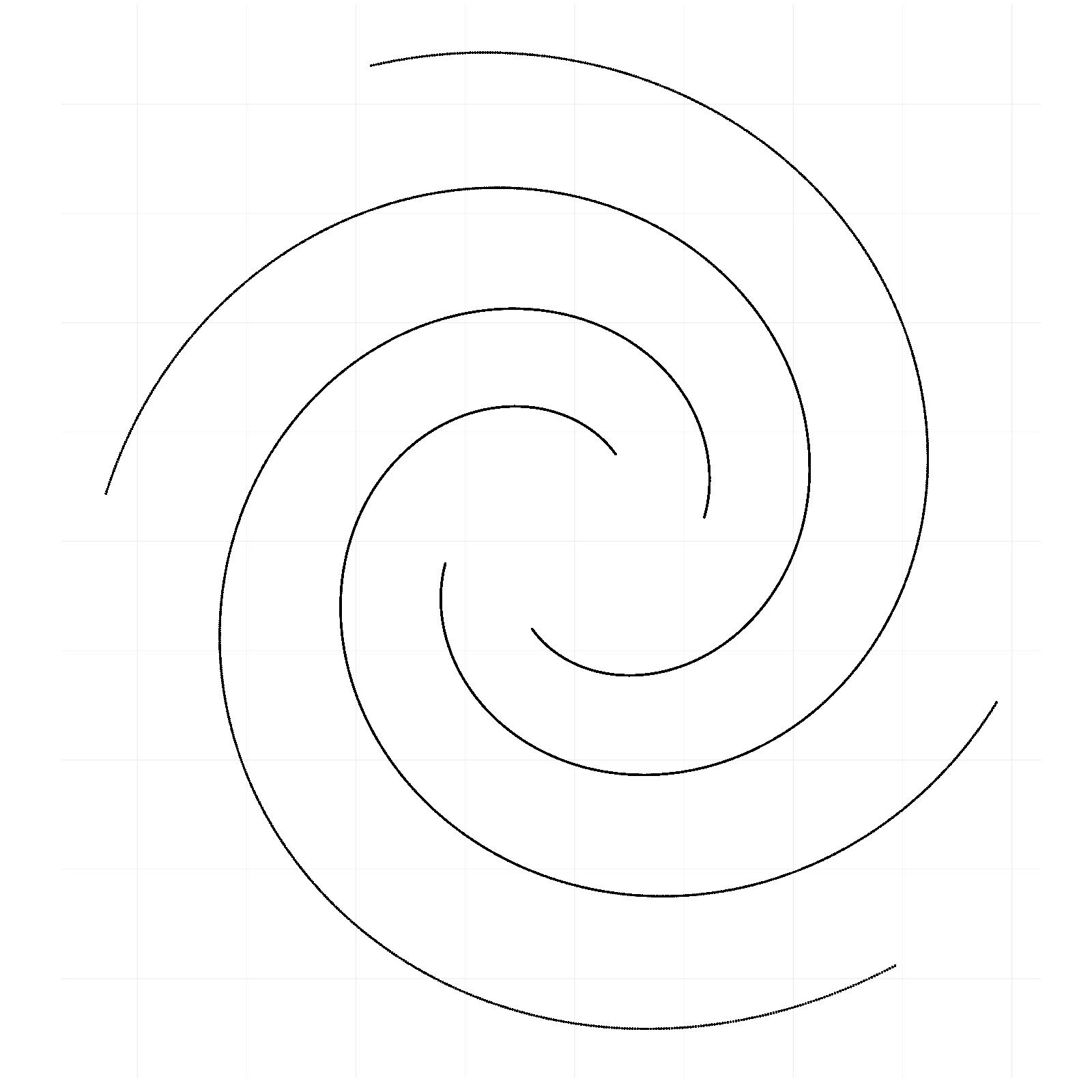
Named after the Greek mathematician, the Archimedean spiral bears a remarkable resemblance to the spiral arms (from a top-down perspective at least) of the Milky Way. In polar coordinates, the curve is given by:

Equivalently, the Cartesian coordinates would be:

In the language of tidyverse, once we have the desired range of $\theta$, the full set of points can be generated by:

spiral_arm <- tibble(
  theta = seq(from = theta_from, to = theta_to, length.out = theta_length)
) %>% 
  mutate(
    r = theta ^ k,
    x = r * cos(theta),
    y = r * sin(theta)
  )

This should get the job done nicely. Now, what if we want more than one spiral arm? One solution would be to repeat the process several times and add a constant to theta for rotation purposes:

spiral_arms <- lapply(
  list(id = seq_len(num_of_arms)),
  function(id, theta_from, theta_to, arm_width){
    tibble(
      id = id,
      theta = seq(from = theta_from, to = theta_to, length.out = theta_length)
    ) %>% 
      mutate(
        r = theta ^ k,
        x = r * cos(theta + 2 * pi * id / num_of_arms),
        y = r * sin(theta + 2 * pi * id / num_of_arms)
      )
  }) %>% 
  bind_rows()

Lo and behold - Archimedes has given us the skeleton upon which a galaxy will be born.

Fleshing out the Skeleton

Stars rarely align on a line. Instead, they exhibit some degree of duality of individual randomness and collective predictability. We can jitter the points vertically and horizontally with some white noises to achieve similar effect. If there aren’t enough points, reuse the exisiting ones!

stars <- sprial_arms %>% 
  slice(rep(row_number(), star_intensity)) %>% 
  mutate(
    x = x + rnorm(n(), sd = width),
    y = y + rnorm(n(), sd = width)
  )

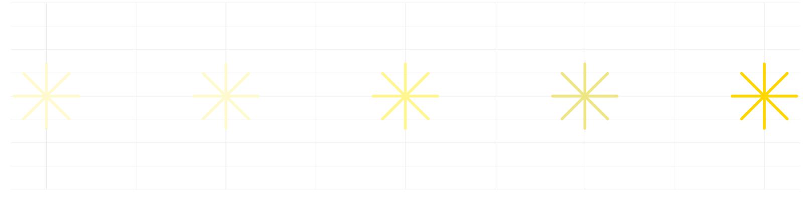
There are two moving pieces in the equation. First, the intensity variable controls overall how many stars will be created. On the other hand, the standard deviation of the noise governs the dispersion of how far a star tends to diverge from its spiral arm. Also, in R’s plotting convention, shape number 8 will give us that star-shaped point we want.

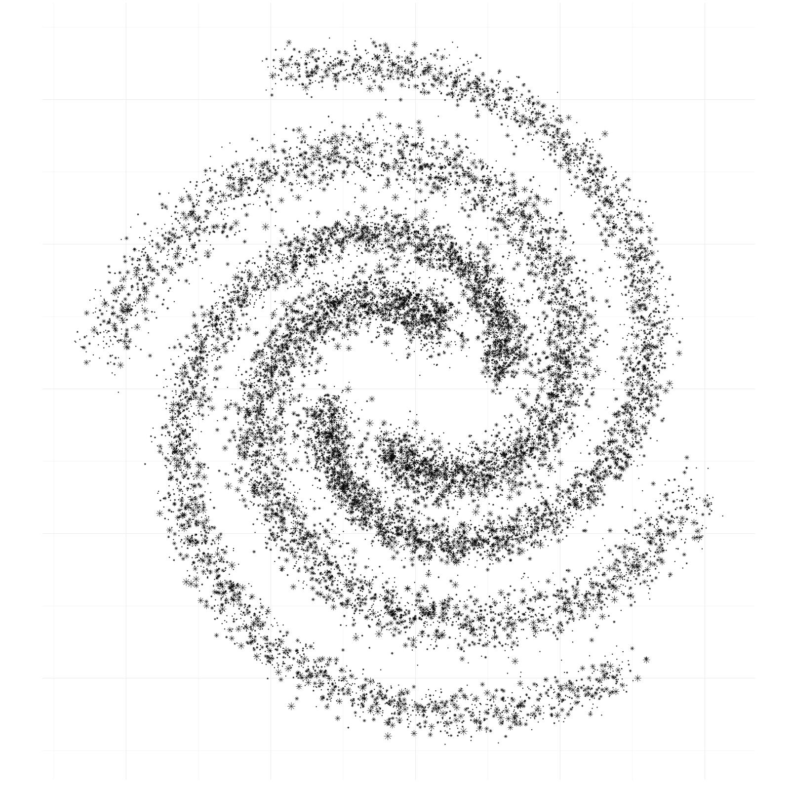
There seems to be one problem though - why don’t the stars shine?

Twinkle Twinkle Little Star

As it turns out, black isn’t the greatest choice of color when it comes to stars. It’s a subjective call but personally, I would rather that they are colored this way:

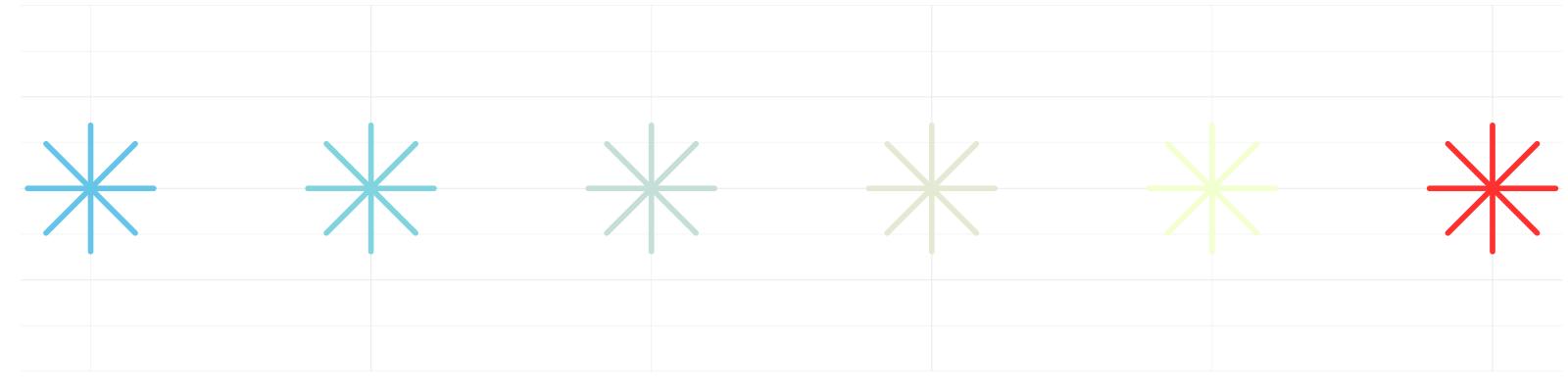
Even then, no color alone can bring the kind of vitality and liveliness that we’ve come to expect from a photo. Ideally, each star should be assigned its own color by randomly sampling from the color space (with replacement):

stars <- stars %>%
  mutate(
    color = star_colors %>% sample(size = n(), replace = TRUE)
  )

In fact, we can further randomize other attributes of the stars as well, i.e., either via sampling values from a predefined set (e.g., random sizes for the stars) or letting it correlate with some feature (e.g., opacity being inversely proportional to the radius from the center). Adding multiple layers of halo effect also helps in terms of introducing the illusion of a vibrant galaxy.

ggplot(sprial_arms, aes(x = x, y = y)) +
  geom_point(data = stars, size = star_halo_size1, color = "white", shape = 8) +
  geom_point(data = stars, size = star_halo_size2, color = "white", shape = 8) +
  geom_point(data = stars, size = stars$size, alpha = stars$alpha, color = stars$color, shape = 8) +
  theme(panel.background = element_rect(fill = background_color))

The halos are effectively nothing more than a few extra points in white at the exact same places, albeit bigger in size and lower in opacity. It’s a simple technique but sometimes it works wonders. When all is being said and drawn, we’ve got ourselves a fairly decent galaxy.

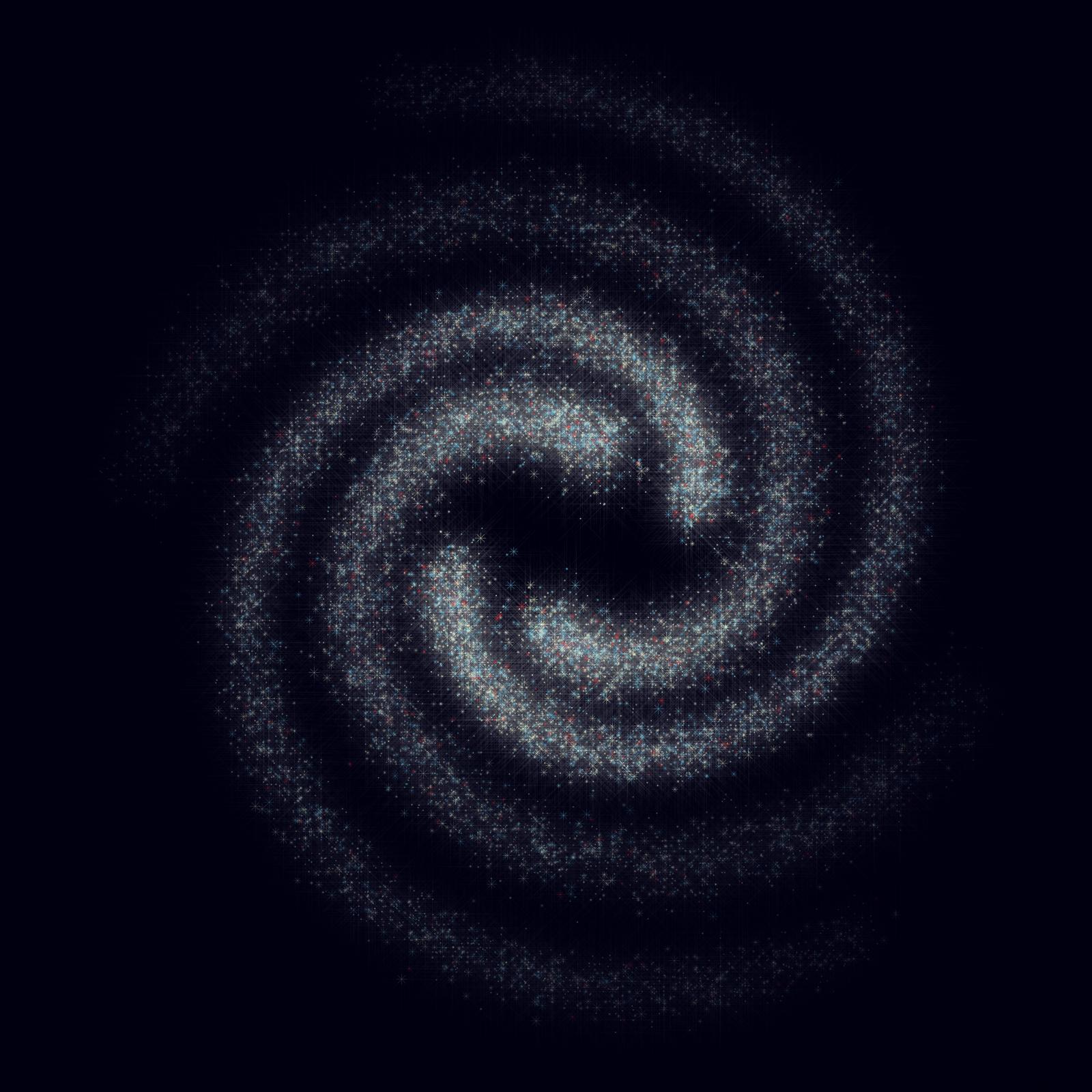
Before we move on, let’s take a moment to appreciate how far we’ve come since sketching the skeleton. However, something is still missing.

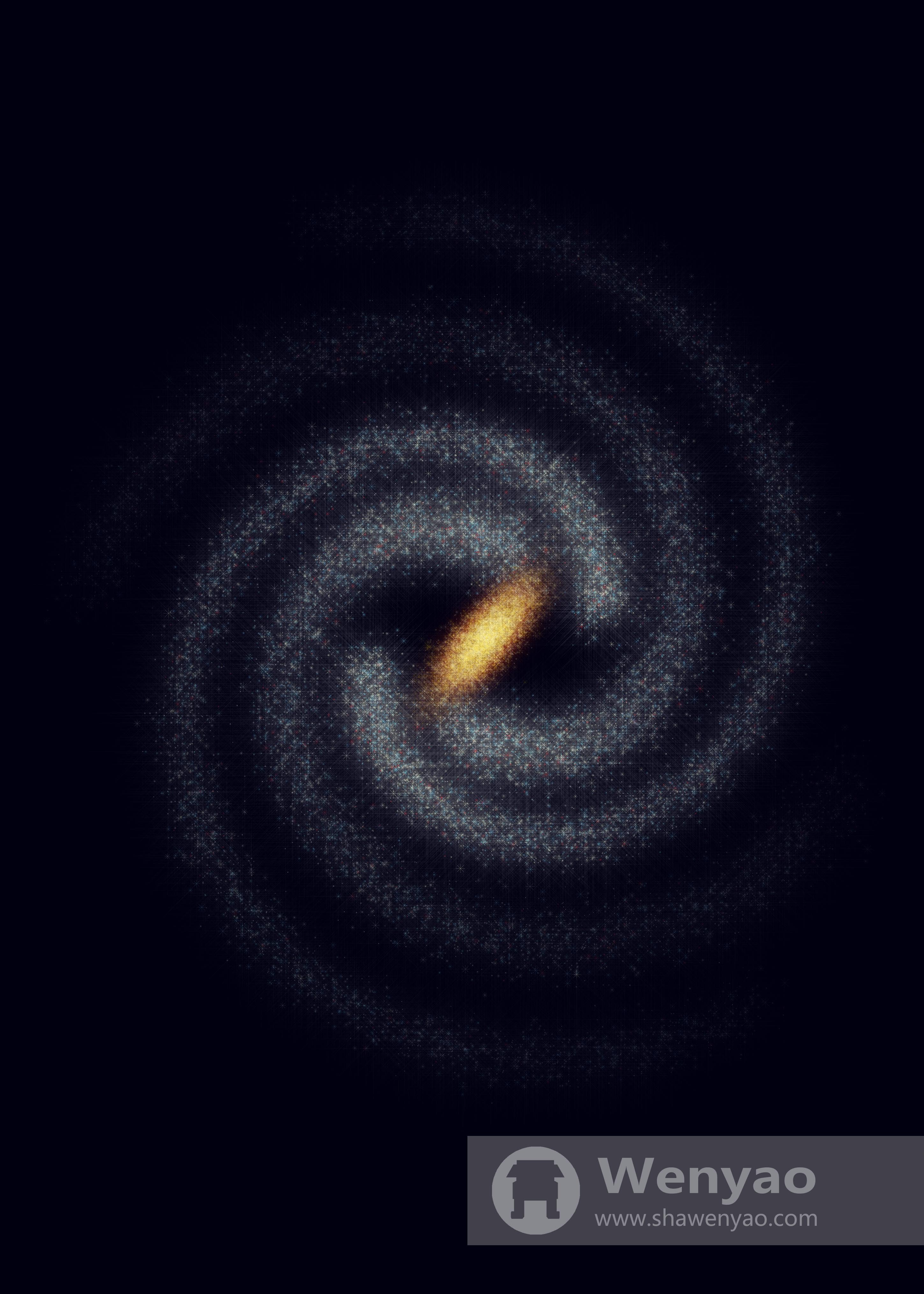
Galactic Center

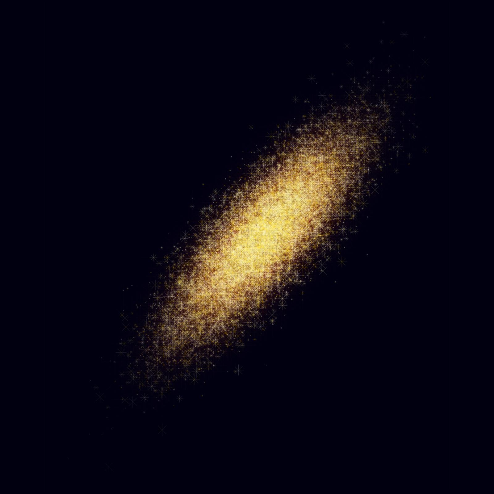
At the heart of the Milky Way lies the brightest region of our galaxy, the Galactic Center, the jewel in the crown. From a purely visual standpoint, it looks like a tilted oval spanning from bottom left to top right, shining and fiery.

But guess what, by no means is it an obscure pattern in geometry. Recall bivariate normal distribution?

where $a$ and $b$ are independent normally distributed random variables. This should give us a way to generate points similar in shape to the Galactic Center:

gc <- tibble(
    x = rnorm(gc_intensity, sd = gc_sd_x)
) %>% 
  mutate(
    y = gc_rho * x + sqrt(1 - gc_rho ^ 2) * rnorm(n(), sd = gc_sd_y)
  )

Again, let’s pick the color palette that best matches that of a burning furnace:

And as usual, we pull the trick of randomized assignment of color, size, transparency in addition to the halo effect:

ggplot(sprial_arms, aes(x = x, y = y)) +
  geom_point(data = gc, size = gc_halo_size1, alpha = gc_halo_alpha1, color = "gold", shape = 8) +
  geom_point(data = gc, size = gc_halo_size2, alpha = gc_halo_alpha2, color = "gold", shape = 8) +
  geom_point(data = gc, size = gc$size, alpha = gc$alpha, color = gc$color, shape = 8) +
  theme(panel.background = element_rect(fill = background_color))

Between you and me, who would have thought that there’s something Gaussian to be found all over the galaxy?

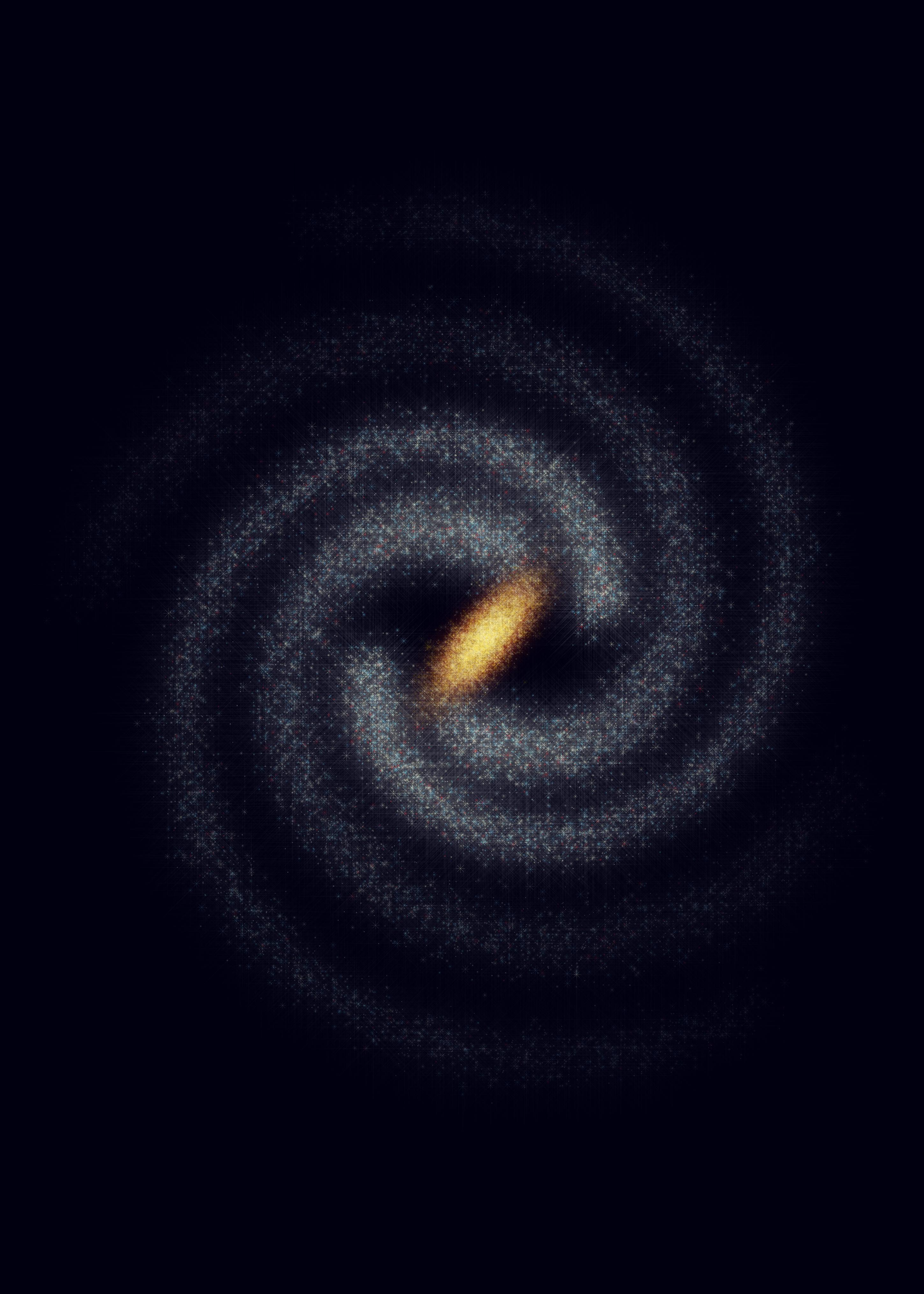
Putting It All Together

From a self-proclaimed data artist who lacks training in cosmology in any meaningful way, the end result works stunningly well. Serene and peaceful, dazzling yet profound, it breathes, chants and whispers, into the void for an eternity. In all fairness, most of the credit goes to our friend randomness who manages to create a sense of guided unpredictability, although not without careful choices of color palette, transparency, shape and size. To do it justice, I highly recommend viewing the image in its native resolution.

Last but not least, the appeal obviously goes beyond the Milky Way. As long as we’ve made up our mind about an object’s functional form (and maybe a new color palette that goes with it), everything else should still hold. This bodes well for other system, constellation or galaxy that we want to give a try so please feel free to let me know if you would like to see Andromeda next.

You can also find animation, video, or source.