Where blockchain meets Brownian motion.

Just like how Bitcoin aims at revolutionizing money, automated market maker (AMM) emerges as the disruptor of traditional exchange. While NYSE and NASDAQ use an order book to achieve price discovery function and balance supply with demand, Uniswap, the biggest decentralized exchange, relies on what’s known as the constant product formula. At the time of writing, Uniswap has over $2.5 billion in total value locked in its liquidity pool according to DeFi Pulse, proving that there is indeed an appetite to end the monopoly of traditional exchange.

One of AMM’s most important divergences from traditional exchange is that it divides its market participants into two distinct roles: liquidity providers and traders. In a nutshell, the former deposits equal value of any pair of assets into the liquidity pool and the latter trades one for the other based on what’s available in the pool. This creates interesting ramifications in terms of risk for the liquidity providers. In this post, we study the characteristics of the price dynamics in Uniswap under the usual assumption that the prices of the underlying asset pair follow a drift-diffusion process. Note that the analysis assumes zero liquidity pool growth (other than due to transaction fees) and zero risk-free rate as well.

Uniswap Explained

Examine the liquidity pool composed of asset $A$ and $B$. For simplicity, let $a_t$ and $b_t$ denote the number of units of $A$ and $B$ available in the liquidity pool respectively. At any point in time, we have:

\[a_t b_t = k\]

This is known as the constant product formula. Since the liquidity pool must have equal value of both assets (one can arbitrage if it doesn’t!), it also implies that the current exchange rate of one unit of asset $A$ in terms asset $B$ is

\[e_t = \frac{ A_t }{ B_t } = \frac{ b_t }{ a_t }\]

where $A_t$ and $B_t$ are the unit prices of asset $A$ and $B$ measured in a common numeraire (be it Bitcoin or US dollar, your choice).

At time $0$, there are $a_0$ units of asset $A$ and $b_0$ units of asset $B$ in the pool. Now, if a new order comes along to buy $\Delta a_1$ units of asset $A$, after the transaction settles, the ending balances in the pool for asset $A$ and $B$ will be:

\[a_1 = a_0 - \Delta a_1\] \[b_1 = \frac{ k }{ a_0 - \Delta a_1 }\]

This leads to a new exchange rate of:

\[e_1 = \frac{ a_0 b_0 }{ (a_0 - \Delta a_1)^2 } = \frac{ a_0^2 }{ (a_0 - \Delta a_1)^2 } \cdot \frac{ b_0 }{ a_0 } > \frac{ b_0 }{ a_0 } = e_0\]

which indicates that asset $A$ has appreciated against asset $B$, as a result of having fulfilled the demand for asset $A$ and the subsequent “scarcity” of it in the pool.

While the individual prices of asset $A$ and $B$ can still very much follow their own dynamics, Uniswap provides a way for traders to express their view on the price of one in terms of the other. In other words, everything is being valued on a relative term in the Uniswap exchange. This setup has a few desirable properties to it. Just to name a few:

• if there’s no trade, the relative price level (i.e., exchange rate) stays at its initial value
• a smaller trade is expected to be fulfilled at the market price of exchange without moving it too much
• a larger trade will move the price substantially along the hyperbolic curve, with the asset in demand appreciating against the other
• a very large trade (e.g., something close to the remaining balance in the pool) will lead to a price impact so prohibitively high that it is close to impossible to deplete the inventory.

In other words, Uniswap appears to achieve infinite market depth with finite supply of assets. Generally, the liquidity provider puts down:

\[v_0 = a_0 A_0 + b_0 B_0\]

amount of money (again, measured in an arbitrary numeraire) today in exchange for:

\[v_t = a_t A_t + b_t B_t\]

at time $t$. By contrast, a buy and hold strategy will have the following payoff at time $t$:

\[v'_t = a_0 A_t + b_0 B_t\]

Price Slippage vs Fee Income

The payoff at time $t$ for liquidity providers can be further decomposed into two parts - capital appreciation (or depreciation) due to price slippage and income from collecting transaction fees.

One on hand, as trades fulfill, newly-arrived supply and demand drive the price away from its starting point. Formerly known as price slippage, this phenomenon can lead to either a gain or loss to the liquidity provider, but it always underperforms a buy and hold strategy (to see why, see appendix). To compensate for the underperformance, AMM usually charges a fee for trading. For example, Uniswap collects 0.3% on every transaction. The fees are put back to the pool right away and every liquidity provider has a pro rata claim on them. As it stands, fee income is effectively the sole incentive for liquidity providers to contribute assets into the pool, compared to simply holding on to the asset pair.

The introduction of transaction fees brings path dependence into the equation. The terminal state alone is no longer sufficient to uniquely determine the payoff to liquidity provider - the path through which it arrives at the ending price also matters. This requires a slight modification to the constant production formula introduced earlier:

\[a_t b_t = a_{ t-1 } b_{ t-1 } + f_t\]

where $f_t$ is the amount of transaction fees collected at time $t$.

Simulation Setup

Assume the prices of asset $A$ and $B$ follow the following dynamics:

\[\frac{ dA_t }{ A_t } = \mu^A dt + \sigma^A dW^A \\ \frac{ dB_t }{ B_t } = \mu^B dt + \sigma^B dW^B \\\]

where $dW^A$ and $dW^B$ are correlated Brownian motions:

\[dW^A dW^B = \rho dt\]

Thanks to the explicit linkage between volume and price specified by the constant product formula, we have everything we need to back out the trading volume it takes to move the price by that much. Ignoring fees, the new price pair $A_t$ and $B_t$ defines how the balances of asset $A$ and $B$ evolve from the time $t-1$ to time $t$:

\[\begin{cases} \frac{ A_t }{ B_t } = \frac{ b'_t }{ a'_t } \\ a'_t b'_t = a_{ t-1 } b_{ t-1 } \\ \end{cases}\]

which yields:

\[\begin{cases} a'_t = \sqrt{ \frac{ a_{ t-1 } b_{ t-1 } A_t }{ B_t } } \\ b'_t = \sqrt{ \frac{ a_{ t-1 } b_{ t-1 } B_t }{ A_t } } \\ \end{cases}\]

After taking transaction fees into consideration, we have the final form of remaining balances in the liquidity pool:

\[\begin{cases} a_t = a'_t + \textbf{ 1 }_{ a_{ t-1 } \geq a'_t } ( a_{ t-1 } - a'_t ) c \\ b_t = b'_t + \textbf{ 1 }_{ a_{ t-1 } < a'_t } ( b_{ t-1 } - b'_t ) c \\ \end{cases}\]

where $c$ is the transaction fee rate and $\textbf{ 1 }$ is the indicator function that takes the value of 1 if the underlying condition is true, or 0 if otherwise. Depending whether the order is to buy asset $A$ with asset $B$ or vice versa, transaction fees can either take the form of asset $A$ or $B$ before being put back to the liquidity pool. More specifically,

• if $a_{ t-1 }$ is greater than $a’_t$, the trader must have purchased asset $A$ with asset $B$, resulting in a decline in the balance of asset $A$ and an increase in that of asset $B$. The protocol retains a portion of the payout (asset $A$) to the trader as transaction fees.
• if $a_{ t-1 }$ is less than $a’_t$, the trader must have purchased asset $B$ with asset $A$, resulting in an decline in the balance of asset $B$ and an increase in that of asset $A$. The protocol retains a portion of the payout (asset $B$) to the trader as transaction fees.

Putting It All Together

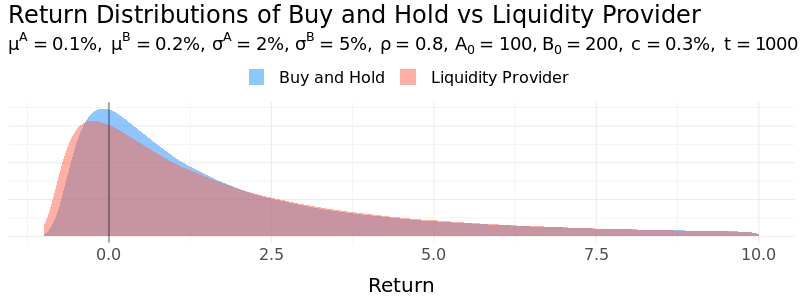
Under a set of arbitrarily-selected parameters, simulation results suggest that even after accounting for transaction fees, the buy and hold strategy still delivers a higher expected return after 1000 steps (transactions). However, acting as the liquidity provider significantly reduces the volatility due to the steady stream of fee income. It also outperforms buy and hold in terms of Sharpe ratio.

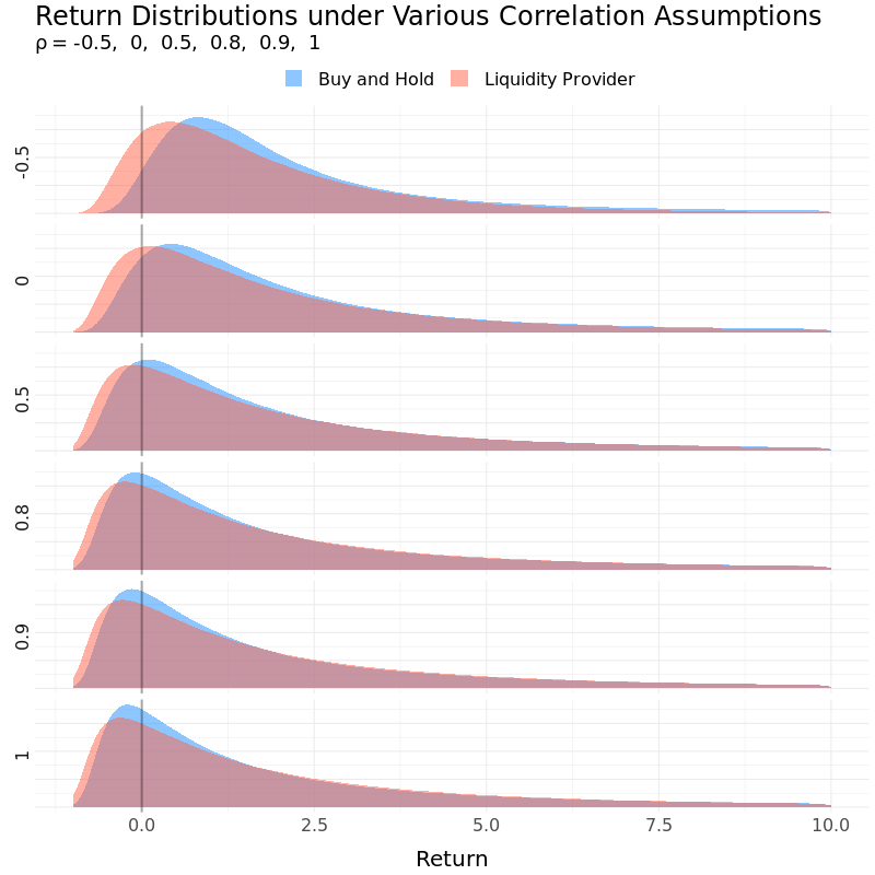
How important is the correlation parameter? Liquidity provider benefits from a low correlation in at least two ways from a mean-variance optimization standpoint. First, the lower the correlation is, the more the two assets’ prices tend to move in opposite directions. The higher level of divergence takes larger amount of trading volume to realize, which should translate into a higher fee income (despite more price slippage). Secondly, a low correlation brings diversification so it’s expected to have lower volatility. All things considered, both expected return and volatility increases as correlation goes up while Sharpe ratio declines. In the extreme case, a correlation of 1 will result in very little price movement in relative terms, to the point where the return dynamics of liquidity provider behave very close to that of a buy and hold.

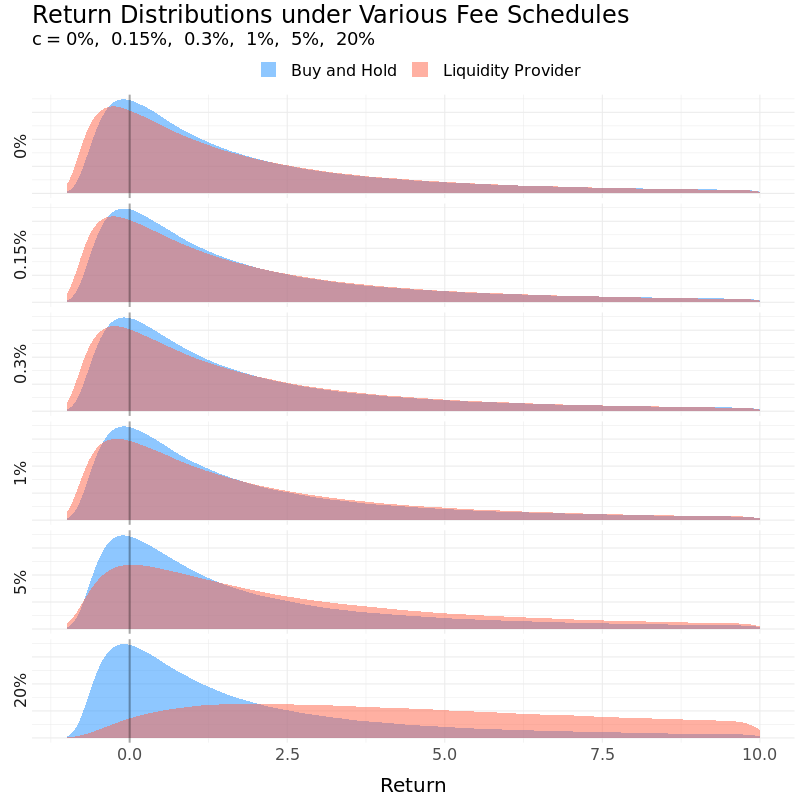
Last but not least, a higher transaction fee rate undoubtedly works in liquidity providers’ favor. All else equal, the higher the fee, the higher the return. Sharpe ratio also improves as the increase in expected return outpaces the increase in volatility.

For details, please refer to the appendix .

Conclusions

If the numerical experiment is any indication, acting as the liquidity provider can often serve as a low-return/low-risk/high-Sharpe-ratio alternative to the buy and hold strategy. In addition, choices of various parameters have subtle yet profound implications on the risk and reward tradeoff and the nature of the underlying asset pairs plays an important role as well.

Uniswap is by no means perfect (especially for those who are targeting an 100% buyout!). However, it opens up an entire new perspective on how we look at the price discovery mechanism. Gone is the order-book-style matchmaking; in its stead is an explicit law that governs the comovement between price and volume. As much as it’s work in progress, let’s take a moment to appreciate how a simple idea can go a long way in the name of decentralized finance.

References

Uniswap. 2020. “How Uniswap works”

Pintail. 2020. “Uniswap: A Good Deal for Liquidity Providers?”

AlfaBlok. 2019. “Risk/Reward of liquidity provision in AMMs”

Appendix

The Effect of Price Slippage

In the absence of transaction fees, compare the terminal values of the two following strategies:

• strategy X: buy and hold
• strategy Y: contribute to liquidity pool

Strategy X’s terminal value is given by:

\[\begin{align} v_t^X &= (a_0 e_t + b_0) B_t \\ % &= (a_0 \frac{ b_t }{ a_t } + b_0) B_t \\ % &= (a_0 \frac{ \frac{ k }{ a_t } }{ a_t } + b_0) B_t \\ % &= (a_0 \frac{ \frac{ a_0 b_0 }{ a_t } }{ a_t } + b_0) B_t \\ &= (\frac{ a_0 ^ 2 }{ a_t^2 } + 1) b_0 B_t \end{align}\]

Meanwhile, strategy Y will have a terminal value of:

\[\begin{align} v_t^Y &= (a_t e_t + b_t) B_t \\ % &= (a_t \frac{ b_t }{ a_t } + b_t) B_t \\ % &= 2b_t B_t \\ % &= 2 \frac{ k B_t }{ a_t } \\ &= \frac{ 2 a_0 b_0 B_t }{ a_t } \\ \end{align}\]

Divide $v_t^X$ by $v_t^Y$,

\[\begin{align} \frac{ v_t^X }{ v_t^Y } &= \frac{ \frac{ a_0 ^ 2 }{ a_t^2 } + 1 }{ \frac{ 2a_0 }{ a_t } } \\ % &= \frac{ \frac{ a_0 }{ a_t } + \frac{ a_t }{ a_0 } }{ 2 } \\ % &= \frac{ a_0^2 + a_t^2 }{ 2 a_0 a_t } \\ % &= \frac{ (a_0 - a_t)^2 + 2 a_0 a_t }{ 2 a_0 a_t } \\ &= \frac{ (a_0 - a_t)^2 }{ 2 a_0 a_t } + 1 \\ &\geq 1 \end{align}\]

As a result, a buy and hold strategy always outperforms being a liquidity provider in the absence of fee income.

Expected Return and Volatility under the Baseline Setup

Strategy	Expected Return	Volatility	Sharpe Ratio
Buy and Hold	4.03	12.72	0.32
Liquidity Provider	2.88	5.56	0.52

Expected Return and Volatility under Various Correlation Assumptions

Strategy	Correlation	Expected Return	Volatility	Sharpe Ratio
Liquidity Provider	-0.5	1.86	2.23	0.83
Liquidity Provider	0	2.22	3.32	0.67
Liquidity Provider	0.5	2.63	4.67	0.56
Liquidity Provider	0.8	2.88	5.56	0.52
Liquidity Provider	0.9	2.98	5.96	0.50
Liquidity Provider	1	3.06	6.18	0.50

Expected Return and Volatility under Various Fee Schedules

Strategy	Fee	Expected Return	Volatility	Sharpe Ratio
Liquidity Provider	0%	2.81	5.51	0.51
Liquidity Provider	0.15%	2.84	5.51	0.52
Liquidity Provider	0.3%	2.88	5.56	0.52
Liquidity Provider	1%	3.09	5.86	0.53
Liquidity Provider	5%	4.48	7.91	0.57
Liquidity Provider	20%	15.36	23.45	0.65

Bold indicates baseline setup.